1 Background

Related to this discussion about measuring errors in volleyball: is it possible to identify the optimal level of aggressiveness in volleyball? Consider serving: if I am too aggressive I will make too many errors; if I am not aggressive enough then my opponent will make perfect passes on my easy serves and consequently win more points with their attack. There ought to be an optimal level of aggressiveness that maximises my point scoring.

My breakpoint rate (i.e. the rate at which I win points when serving) depends on several things:

1. Errors. Obviously I lose the point if I make a service error. My error rate should increase with increased aggressiveness.

2. Aces. My ace rate should also increase with increased aggressiveness, but probably only to a point. If I become extremely aggressive, I will tend to make more service errors and my ace rate will decrease.

3. If the serve is neither an ace nor an error, then my win rate depends on my opponent’s sideout ability. Arguably, increased serve aggressiveness should decrease my opponent’s sideout ability, because their passing and subsequent offense should not be as effective.

A previous study [1] looked at these factors and showed that there is an optimal level of serving aggressiveness that maximises point scoring. We can replicate their findings but using a simpler analysis technique.

2 Processing

We use serving data from the 2015/16 Polish PlusLiga. For each individual player (using only players who had made at least 20 serves) we calculate their error, ace, and opponent sideout rates. We don’t have any direct measure of aggressiveness in the data but if it is genuinely an underlying controller of serve performance then we should nevertheless be able to see its effects. These three variables (error, ace, and opponent sideout rate) should vary in synchrony with aggressiveness. In effect, our data has been measured in three dimensions but the majority of the variation will occur along a single axis (aggressiveness) that is embedded in that three-dimensional data space.

We use a technique known as principal components analysis to recover that hidden aggressiveness axis. This takes our our original dataset and transforms it to a new coordinate system. The first axis of this new coordinate system is chosen mathematically so that it aligns with the direction of maximum variance in the data. The second axis is orthogonal to the first and is aligned with the direction of next-highest variance, and so on.

By our logic above, the largest variations in the data should correspond to variations in aggressiveness, and therefore we might expect the first principal component axis to reflect aggressiveness.

3 Results

We plot error, ace, and opponent sideout rate against the recovered “aggressiveness” axis. The points in each plot represent individual players (with the colour of each point indicating whether that player tends to jump serve or not). The black lines show a smooth fit that gives an indication of the shape of the relationship in question. The grey shading shows the uncertainty around that shape. Note that the numerical scale of aggressiveness (ranging from about -0.2 to +0.3) is an arbitrary one — the numbers have no direct physical intepretation. But different players can be ranked according to their scores on that scale.

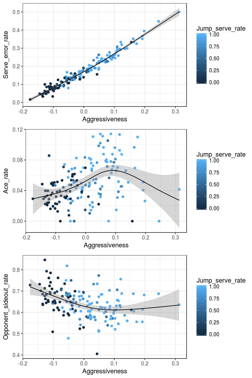
The shapes of these relationships are much as we expected: error rate increases with aggressiveness, and this is a very tight relationship. Ace rate shows a peaked relationship, initially increasing with aggressiveness but falling off again at high aggressiveness values. This is also a weaker relationship that was the case for error rate (i.e. the points are scatted more variably around the line, indicating the influence of other factors on ace rate). Opponent sideout rate decreases with aggressiveness, and flattening out (or even perhaps increasing slightly) at high aggressiveness values.

While we did not use any information about breakpoint rate to construct our aggressiveness axis, we can nevertheless plot aggressiveness against breakpoint rate:

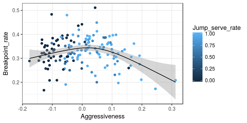
This curve peaks at middling values of aggressiveness — around 0.02 — so there does indeed appear to be an optimal aggressivess level at which point scoring is maximised. This aggressiveness level corresponds to a serve error rate of around 0.19. Individual player scores could be used to help tailor their serving strategy. The curve appears to be asymmetric, rising relatively slowly as aggressiveness increases, before dropping more sharply. Thus it would seem that it is better to err on the side of caution (there is less of a penalty to being over-cautious than there is to being over-aggressive).

4 Postscript

Since breakpoint rate has an optimal aggression level, and aggression is tightly (monotonically) related to serve error rate, it follows that we should also see the same optimal breakpoint rate if we plot it directly against serve error rate:

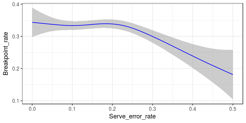
This curve is a very similar shape to the previous one. For practical purposes it may be sufficient simply to assess serve error rate against breakpoint rate in order to explore the optimal level of aggressiveness.

[1] Burton T, Powers S (2015) A linear model for estimating optimal service error fraction in volleyball. Journal of Quantitative Analysis in Sports 11:117–129. doi:10.1515/jqas-2014-0087