
Adjusted attack indicators
2018-03-12
There are a number of different statistics that are used to assess volleyball attack performance, such as kill rate, attack efficiency, and rally win rate. See for example this article and some related discussion.
Different indicators offer insights into different facets of attacking, but most tend to suffer from “opportunity bias”: the value of a statistic for an individual player is influenced by the attack opportunities that the player has been given. An attacker who generally spikes in difficult situations will likely have lower attack success compared to an attacker who gets easier opportunities.
We can illustrate this with some data from the 2016/17 Polish PlusLiga. The table below summarizes the three most common attack types for outside hitters: V5 (highball to position 4), X5 (a faster-tempo set to 4 — this is the standard outside attack), and XP (backrow pipe attack). The mean kill rate of these attacks is shown, for both serve-reception phase and transition phase attacks.
| Attack code | Phase | N | Kill rate |
|---|---|---|---|
| V5 | Reception | 1885 | 0.312 |
| V5 | Transition | 2410 | 0.322 |
| X5 | Reception | 5687 | 0.514 |
| X5 | Transition | 2542 | 0.459 |
| XP | Reception | 1225 | 0.633 |
| XP | Transition | 686 | 0.563 |
X5 and XP attacks are more commonly used in reception phase than in transition, and have a higher kill rate in reception phase. Highball V5 attacks are more commonly used in transition than in reception, and have the lowest kill rate. An attacker who gets set more high balls or transition balls than other attackers might look worse in terms of raw attack rate, not necessarily because they are a weaker attacker but because they are typically hitting in more difficult situations.
Can we correct for opportunity on the basis of attack type and play phase?
Kill rates by attack type and play phase
Let’s look at two players, both outside hitters. Player 1 has a raw kill rate of 0.461, and player 2’s is very similar at 0.465.
However, if we look at their X5/V5/XP attack breakdown …
| Attack code | Phase | Player 1 attack percentage | Player 2 attack percentage |
|---|---|---|---|
| V5 | Reception | 6.7 | 8.5 |
| V5 | Transition | 21.2 | 16.0 |
| X5 | Reception | 27.9 | 34.0 |
| X5 | Transition | 18.8 | 14.5 |
| XP | Reception | 4.8 | 7.0 |
| XP | Transition | 4.8 | 4.0 |
… we can see that player 1 has fewer X5 reception attacks, and a greater proportion of V5 attacks. Thus, even if these two players had identical hitting ability we would expect player 2’s raw kill rate to be higher. If we wanted to compare those two players, it would be helpful if we could adjust their kill rates to reflect their respective opportunities.
The adjustment procedure is fairly straightforward:
- Choose the “opportunity” variables by which to adjust the attack indicator. Here we use attack code and phase, as in the above tables1. Each different combination of these variables defines an adjustment category (e.g. “X5 reception”, “X5 transition”, “V5 reception”, etc).
- Calculate the league-average proportion of attacks in each of these categories. For example, in our demonstration data, “X5 reception” attacks constituted 30.2% of all attacks by outside hitters.
- Then for each player:
- Calculate the player’s kill rate in each of those same adjustment categories.
- Combine those rates using a weighted average, where the weightings are the league-average proportions calculated in step 2.
This gives an “adjusted” kill rate, which effectively acts as if all attackers had the same attack opportunities (same number of attacks in each of the different categories).
With our two example players, the adjusted rates are 0.493 for player 1 and 0.459 for player 2. Their raw rates were similar but player 1 generally had more difficult opportunities, and so his adjusted rate is higher than for player 2.
So what does this look like for the whole league? The raw and adjusted kill rates for all attackers (that had at least 20 attacks in total) are shown below:
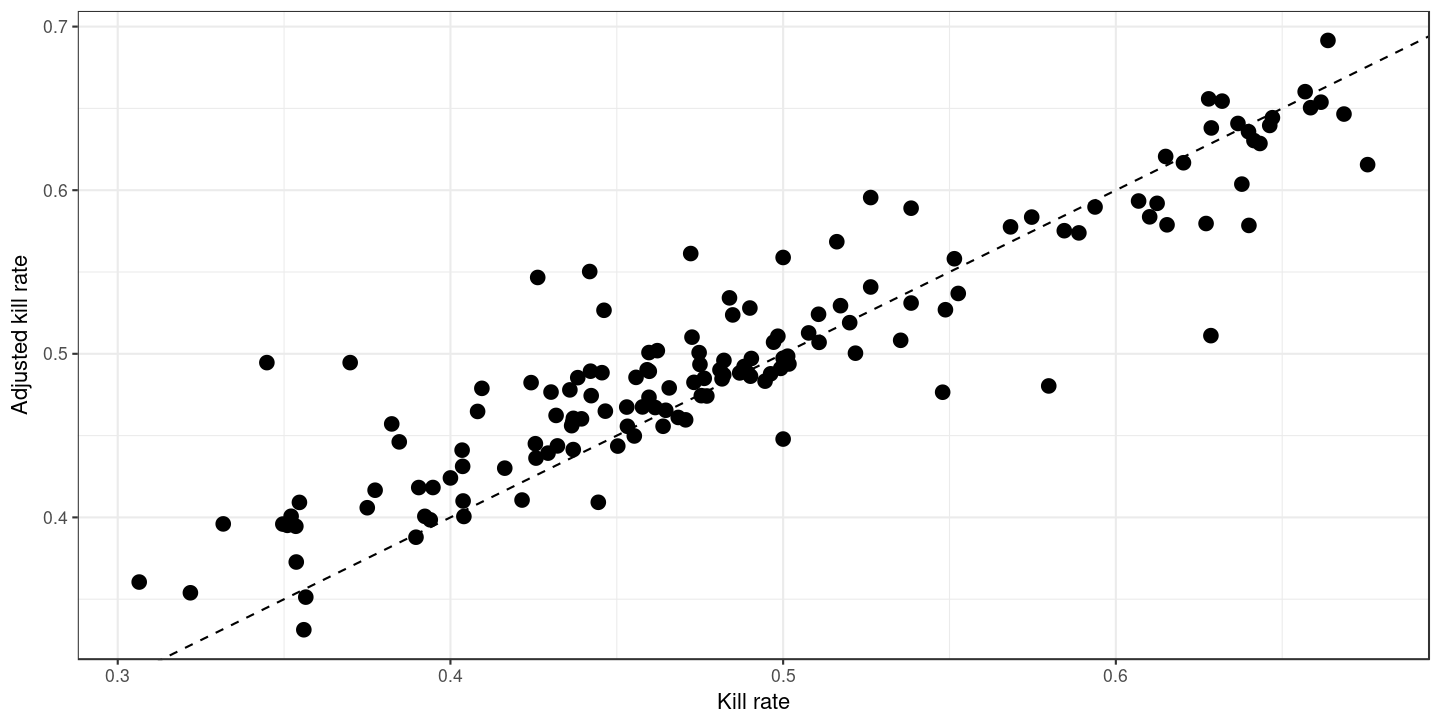
The dashed line is the 1:1 line. If the adjustment did nothing, all the points would lie exactly on this line. We can see that points on the left generaly lie on or above the line (meaning that players with low kill rates tend to be adjusted upwards). Similarly, points on the right tend to lie on or below the line: players with high kill rates tend to be adjusted downwards.
This is what we would expect: some players have a genuinely high raw kill rate and won’t be adjusted much, but others have an inflated kill rate through good opportunities and perhaps low total attack attempts. The kill rate for these players will typically be adjusted downwards.
One tricky aspect of this procedure is dealing with small sample sizes. We are looking at proportions (the number of kills from the number of attempts), and these numbers can be small in some cases, such as rarely-used attack types. Let’s say an attacker achieved two kills from two attempts of a certain attack type: that’s a 100% kill rate! However, their true kill rate for these attacks is unlikely to be 100%, and using such extremely-high (or extremely-low) values in the calculations tends to distort the results. A simple but perhaps crude solution to this might be to exclude categories for a particular player where the numbers are small2. A less cavalier solution is to use a statistical model3 that gives us not only an estimate of each kill rate but also its associated uncertainty. Rates based on small sample sizes will tend to have high uncertainty, and are given less importance in the adjusted result.
Of course, this kind of correction isn’t foolproof. Maybe player 1 in our example has typically been selected to play against weaker opposing teams, when his team’s main hitters are being rested (in which case perhaps we could correct for opponent strength?). But maybe also there are other, more subtle factors at play that aren’t apparent in the data and can’t be corrected for.
This kill rate adjustment has been implemented in the analysis and reporting app.
In order to use attack type as the basis for the correction, we need to be confident that the matches in our data set have all been scouted with consistent attack codes. If attack codes are not consistent, it might be reasonable to use the scouted attack start zone and tempo (quick/tense/high/etc) instead of attack type (code). Reception or set quality could also be used as a basis for correction, but these have the drawback of being subjective assessments, and may also not be consistent across different scouts and matches.↩
Some categories might be sensible to exclude anyway, such as attacks on overpasses or attack types that are rarely used by any team.↩
A binomial generalized linear model of the form
kill~phase:attack_type. Having fitted the model, we simulate from the model in each of the adjustment categories, with the number of samples in the different categories following the league-average proportions. The “adjusted” statistic is the average of these values.↩