
Comparing setters
2019-03-23
Ben Raymond, Mark Lebedew, Adrien Ickowicz.
Different setters use different strategies in choosing which attackers they set at what times. These include:
- setting the attackers that are getting the most kills (these might the be best attackers, or the attackers facing the weakest blockers, or both)
- isolation and other tactics that make it difficult for the defence (particularly the opposition middle blocker) to predict where the set is going, and to put up an effective defence (block).
In this series of posts we will look at two characteristics of a setter’s strategy: predictability, and their tendency to set the attacker with the best kill percentage.
Comparing setters - predictability
Let’s start with predictability, and initially we’ll ignore the sequence of sets that a setter makes. We’ll just look at their overall set distribution.
Throughout these analyses, we use only reception-phase sets, on good or perfect passes. Sets are classified as “L” (left-side), “R” (right-side) “1T” (first-tempo (quick) attacks), or “P” (pipes). We only include setters with more than 100 sets in total.
Predictability without considering sequence order
We summarize a setter’s overall distribution by calculating the proportion of sets they made in each of our four categories. So, for example, a setter who sets left- and right-side sets (in equal numbers) would have a distribution of [0.5 0.5 0.0 0.0] whereas a setter who sets equal numbers of sets in all four categories would have a distribution of [0.25 0.25 0.25 0.25].
We can quantify the predictability in this distribution using a quantity called information entropy. Information entropy (also known as Shannon entropy) has its roots in information theory, and is a measure of the amount of information in a message. This might sound like a strange thing for us to be interested in, but it is useful because it tells us about the predictability of the setter. The “message” in our case comprises the set choices that a setter makes. A setter who only ever sets one type of set would have an entropy of 0, because there is no information in this message (their set choice never changes). This setter is also completely predictable: we will always know where they are going to set. A setter who sets left- and right-side sets in equal numbers has some information in their distribution (the set choice does change back and forth between the two possibilities) and has an entropy of 1. A setter who sets equal numbers of sets in all four categories has the maximum entropy of 2. This last setter is also the least predictable, in the sense that any given set is just as likely to go to any of the four options.
Real data
Let’s look at some real data, taken from the 2018 Men’s Volleyball Nations League. We calculate the entropy for each setter in each rotation (position on court) and then average across rotations to get a single entropy value per setter.
The top 5 setters according to their entropy:
| Player | Team | Total number of sets | Entropy | L | 1T | R | Pipe |
|---|---|---|---|---|---|---|---|
| BENJAMIN TONIUTTI | FRANCE | 345 | 1.92 | 0.22 | 0.32 | 0.30 | 0.16 |
| Micah Christenson | USA | 420 | 1.90 | 0.24 | 0.37 | 0.22 | 0.17 |
| Tyler SANDERS | CANADA | 362 | 1.89 | 0.22 | 0.34 | 0.30 | 0.14 |
| NAONOBU FUJII | JAPAN | 255 | 1.86 | 0.23 | 0.36 | 0.29 | 0.12 |
| HARRISON PEACOCK | AUSTRALIA | 325 | 1.86 | 0.28 | 0.32 | 0.30 | 0.10 |
| Player | Team | Total number of sets | Entropy | L | 1T | R | Pipe |
|---|---|---|---|---|---|---|---|
| Meng Liu | CHINA | 115 | 1.67 | 0.17 | 0.37 | 0.36 | 0.10 |
| IVAN KOSTIC | SERBIA | 169 | 1.67 | 0.31 | 0.32 | 0.34 | 0.04 |
| MICHELE BARANOWICZ | ITALY | 135 | 1.65 | 0.39 | 0.31 | 0.24 | 0.06 |
| Igor KOBZAR | RUSSIA | 273 | 1.56 | 0.23 | 0.49 | 0.23 | 0.05 |
| Dmitry KOVALEV | RUSSIA | 148 | 1.55 | 0.23 | 0.46 | 0.30 | 0.01 |
The setters with the highest entropy tend to have relatively even usage across the set categories, whereas those with lower entropy tend to favour one or more categories more heavily.
This approach can be extended to take the ordering of a setter’s choices into account, as well as their overall distribution.
Considering sequence order
So far we have just looked at a setter’s overall distribution (their proportion of sets in each of the four categories), but ignored the sequence in which those sets were made. We can add a temporal aspect to this process by looking at pairs of sets in sequence. For example, if a setter made the sequence of sets L, L, L, 1T, L, R, this can be broken into the pairs L/L, L/1T, 1T/L, and L/R (order matters, so L/1T and 1T/L are not the same as each other). We can then use these pairs as the basis of our distribution, and tabulate it as before — so in this example, 40% (2 of 5) pairs were L/L, and the remainder (L/1T, 1T/L, and L/R) each occurred once (20%).
From this we can calculate entropy (let’s call this “sequence entropy” to distinguish it from entropy calculated without considering sequence order). The sequence entropy gives us some insight into the predictability of a setter’s choice given the last set that they made.
Some examples:
| Sequence | Entropy | Sequence entropy |
|---|---|---|
| L, R, L, R, L, R, L, R, L | 0.99 | 1.00 |
| L, L, L, L, R, R, R, R, L | 0.99 | 1.81 |
| L, L, R, R, L, L, R, R, L | 0.99 | 2.00 |
These three examples each contain five L’s and four R’s, and so all have the same entropy value of 0.99 (ignoring sequence order). However, if we take sequence order into account, the sequence entropy values differ. The first example sequence contains only two pairs (L/R and R/L) and has the lowest sequence entropy of the three examples. A set to L is always followed by a set to R, and vice-versa. The second contains contains four pairs (L/L, L/R, R/R, R/L), and so its sequence entropy is higher than the first example — but note that L/L and R/R appear more often than L/R and R/L. This makes it more predictable (because if we just guessed that L always follows L and R always follows R, we’d be right 6 out of 8 times). The third example also contains four pairs, and in this case they occur equally often, and so its sequence entropy is the highest of the three.
We can extend this approach to higher-order patterns, by looking at sub-sequences of three sets (second-order patterns), four sets (third-order), and so on. Here we use sub-sequences from length two to length five, and average these entropies to get an overall measure of sequence entropy. (Note: what we are calling “sequence entropy” is known in the literature as “permutation entropy”1).
Real data
Let’s look again at the data from the 2018 Men’s Volleyball Nations League.
The top 5 setters according to their sequence entropy:
| Player | Team | Total number of sets | Sequence entropy |
|---|---|---|---|
| Maximiliano Cavanna | ARGENTINA | 571 | 5.46 |
| MIR SAEID MAROUFLAKRANI | IRAN | 502 | 5.32 |
| Micah Christenson | USA | 420 | 5.26 |
| NIKOLA JOVOVIC | SERBIA | 364 | 5.10 |
| Georgi Seganov | BULGARIA | 420 | 5.09 |
And a plot of entropy (ignoring sequence) against sequence entropy for all players:
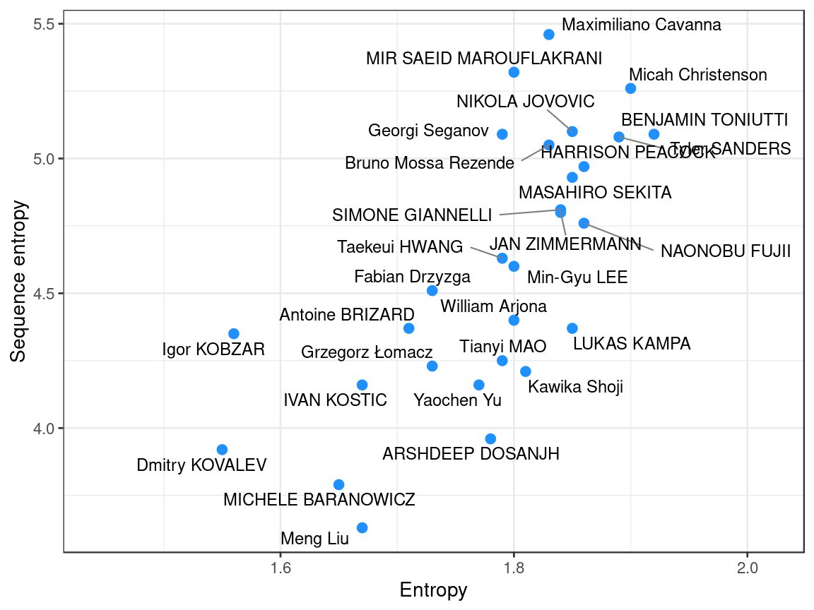
Marouf and Cavanna had the highest values of sequence entropy, and yet both showed only moderate entropy without considering sequence. This suggests that while their sequences showed variety, their overall distributions remained somewhat biased towards particular set choices. In contrast, others (Kampa, Shoji, Fuji, Dosanjh) ranked considerably lower on sequence entropy relative to their entropy, indicating that while their overall distributions were relatively balanced, their sequences were more predictable than other setters. A few setters (notably Christenson, Toniutti, Sanders, Jovovic) were high on both measures.
It’s not clear from these initial results whether one of these entropy measures is more useful than the other, or what the differences between them really mean from a practical perspective. For the time being at least, we’ll continue to look at both.
Maximizing kills
In the previous section we looked at entropy as a way of assessing the predictability and variety of a setter’s distribution patterns. However, not all setters necessarily strive to maximize their unpredictability. An alternative tactic might simply be to set to the attackers who are getting the most kills.
We can get a handle on this strategy by looking at the overall kill rate on a setter’s sets, and compare it to the kill rate that we would expect to see if the setter chose their target attacker at random. The latter can be calculated from the average kill rate of each attack type in each rotation. We calculate the ratio of the actual to expected kill rate and refer to this as the “kill rate priority”. A setter who is not actively seeking to maximize kill rate should have a lower kill rate priority than a setter whose strategy is focused on maximizing kill rate.
The top few setters by kill rate priority:
| Player | Team | Total number of sets | Kill rate priority |
|---|---|---|---|
| Meng Liu | CHINA | 115 | 1.146 |
| Antoine BRIZARD | FRANCE | 195 | 1.121 |
| MICHELE BARANOWICZ | ITALY | 135 | 1.101 |
| Igor KOBZAR | RUSSIA | 273 | 1.092 |
| Dmitry KOVALEV | RUSSIA | 148 | 1.088 |
Most of these setters were towards the bottom of the list when ranked by entropy. Indeed, if we plot kill rate priority against entropy we can see that these are negatively related:
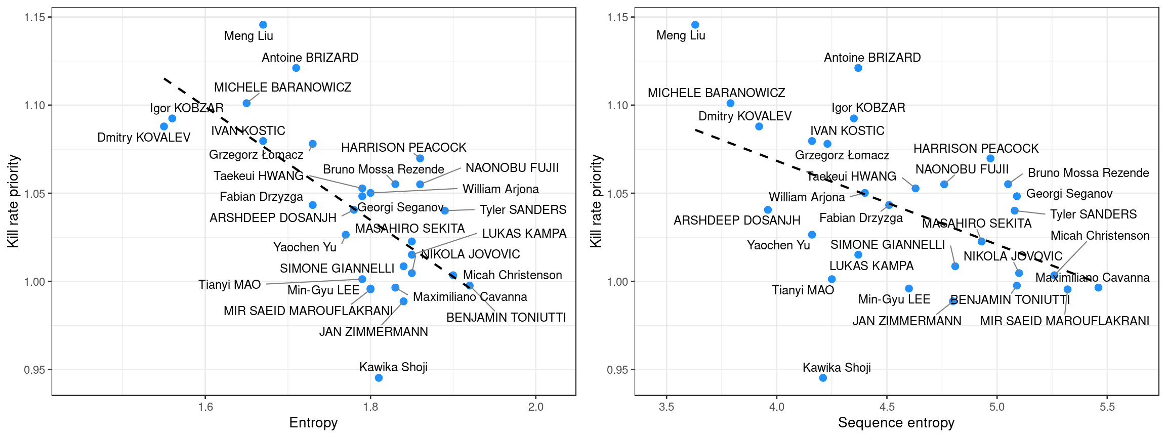
The fact that these relationships are negative makes sense: it’s generally not going to be possible to set all attack types equally (hence maximising entropy) while at the same time preferring to set to the best attackers.
In the next post, we’ll look at the implications of these two setting strategies, and whether we can see in the data that these two strategies lead to differences on court.
Bandt C & Pompe B (2002) Permutation entropy: a natural complexity measure for time series. 10.1103/PhysRevLett.88.174102↩