
How to judge a setter’s setting choices
2020-12-30
Adrien Ickowicz with Ben Raymond, Mark Lebedew, and Chad Gordon.
It started as a casual conversation with one of the players I had the chance of coaching. Following a game with a disappointing result, but not a bad on-court performance, we followed up with a debrief with the players. We went through (almost) every aspect of the game. Well, bar one, according to that player. We forgot to mention the setter’s performance. I initially started to explain why it was difficult to evaluate the setter beyond a simple quality assessment of the set, or using a few statistical indicators such as kill and point win rates. But the next question was: how about the choices? Yes, you have them indirectly through these indicators, but is there another way? In a previous article we looked at ways of characterizing setter strategies, but this does not really lend itself to making quantitative assessments of how well a setter chooses the attackers they set. Following a night of extremely agitated sleep while this idea was running amok in my brain, I decided to have a go at it.
Perhaps surprisingly, an answer lies in something called the multi-armed bandit problem. Yes, as in Las Vegas slot machines.

From a research statistician point of view, that problem can be described as:
The multi-armed bandit problem is a reinforcement learning example where we are given a slot machine with n arms (bandits) with each arm having its own rigged probability distribution of success. Our objective is to pull the arms one-by-one in sequence such that we maximize our total reward collected in the long run. The non-triviality of the multi-armed bandit problem lies in the fact that we (the agent) cannot access the true bandit probability distributions. All learning is carried out via the means of trial-and-error and value estimation. So the question is: How can we design a systematic strategy that adapts to these stochastic rewards?
This sounds remarkably similar to the problem faced by the setter. While he surely has some idea of how well each of his hitters is likely to perform before the game even starts, he doesn’t know exactly. Actual performances will depend on the opposition, how each hitter is playing on the day, and other factors. So the setter’s challenge is to explore his hitting options and evaluate their relative success rates, while simultaneously tailoring his setting strategy to maximize the team’s overall point win rate.
Let’s first define the problem in volleyball terms. At any given time, the setter makes a choice of attack type (X1, X2, etc…) he thinks is most likely to score the point. Sometimes, especially early in the game, a bit of exploration and clever randomness also prevails, in order to find out which hitters are hitting well and perhaps to keep the other team from predicting what tactics are being used.
Let’s dig in to an example straight away to clarify the thought process. We use data from the Polish PlusLiga 2019-2020 season, and take a look at a given game, say Jastrzębski Węgiel vs MKS Ślepsk Malow Suwałki. In particular, we are interested in the setter choices from Jastrzębski Węgiel, so the first thing to do is for every rotation of the setter, assess the choices made and their respective kill rate:
Rotation | Pass quality | V5 | X5 | X6 | XC | PP | V8 | X7 | X8 | XP | V6 | X1 |
1 | - | 0 (n=2) | 1 (n=1) | |||||||||
1 | ! | 0 (n=1) | 0.33 (n=3) | |||||||||
2 | # | 0 (n=1) | 1 (n=1) | |||||||||
2 | - | 1 (n=1) | ||||||||||
2 | + | 1 (n=1) | 0 (n=2) | 1 (n=1) | 0 (n=1) | |||||||
3 | - | 0 (n=1) | ||||||||||
3 | ! | 0.5 (n=2) | ||||||||||
3 | # | 0.5 (n=2) | 0.5 (n=2) | |||||||||
4 | + | 1 (n=2) | 1 (n=1) | 1 (n=1) | ||||||||
4 | ! | 0 (n=1) | ||||||||||
4 | # | 1 (n=1) | ||||||||||
5 | - | 0 (n=2) | 0 (n=1) | 0 (n=1) | ||||||||
5 | + | 1 (n=1) | 0.67 (n=3) | 0.5 (n=2) | ||||||||
5 | ! | 0 (n=1) | 0 (n=3) | |||||||||
6 | - | 0 (n=1) | 0 (n=2) | 1 (n=1) | ||||||||
6 | ! | 0.5 (n=2) | 0 (n=1) | |||||||||
6 | + | 0 (n=2) | 1 (n=1) | |||||||||
6 | # | 1 (n=1) |
So, this table gives us the kill rate for every possible reception situation the setter faced in that game (reception quality, rotation, attack code — we will omit setter calls, which may be included but will require more data). The n numbers are small because we are looking at sets on serve reception only, from a single match.
Based on that information, we can compare what the sum of the kill rates gives us for every choice made by the setter and the actual points scored. In this instance, the team scored 22 kills from their reception attack.
Now the question is, could the setter have made better choices in this game? Is there an “optimal” setting strategy, and would this have scored better? Remember that the setter does not know the kill rates of the different attack types prior to playing the game (even though he may have an idea).
As it happens, this is a question of high interest in the statistical research community, and it is fairly well studied. And there is one algorithm that is generally accepted to give a fairly optimal solution. It is called … (drumrolls) … the Bayesian Bandit.

What does this criminal algorithm do? Simply it starts by assuming a certain probability of success for a given action, then once the arm is pulled, it looks at the outcome and updates its expected probability of success is for that action. Oh, and also, it does not pick the action with the highest success probability every time, but instead randomly chooses one action, where the probability of choosing is a function of past successes. This allows the algorithm to explore the various choices available and update what it thinks the expected success of each will be (see e.g. this article for a more in-depth explanation of the algorithm). It is nice, elegant, and easy to code. So we do.
The result is in: the bandit setter scored on average 25.1 kills off the attacks. Which is a fraction better than the 22 points that our real setter actually achieved in the game. However, because the Bayesian bandit setter is stochastic by nature, it will not score 25.1 points every time. In fact 90% of the time, the bandit had a score between 21.0 and 29.0 points — so our real setter’s performance was well within the range that we might expect to see from this optimal setting strategy.
Can we push the analysis further? Absolutely. Let’s compare the ‘trajectory’ of the points scored over the course of the match (the vertical dashed lines indicate the ends of each of the three sets):
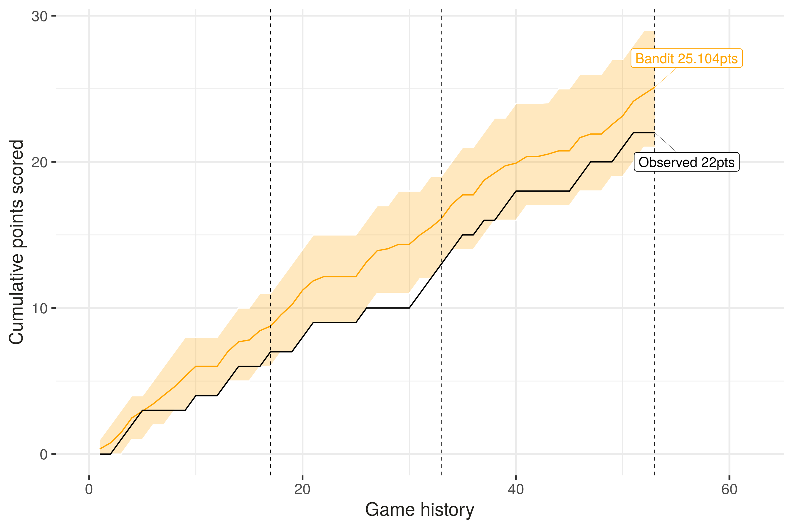
What does it tell us? Well, that potentially in the middle stage of the 1st set the bandit-led team outperformed the setter-led team, and in the beginning of the 3rd, the setter performed well compared to the bandit. Whether our setter’s strategy was good enough to win the match is another question, perhaps for another day, but nevertheless I now have a quantitative basis on which I can evaluate my setter’s performance in terms of the choices they made (not just on their technical skill execution alone).
Finally, before we finish this post, one last question: did our setter make any unexpected choices? That is, if we run a large number of simulations of the bandit setter, were there choices made by the setter that were not (or only rarely) made by the bandit? The way to do it is to simulate step by step, and give the bandit setter the same information as the setter of the team.
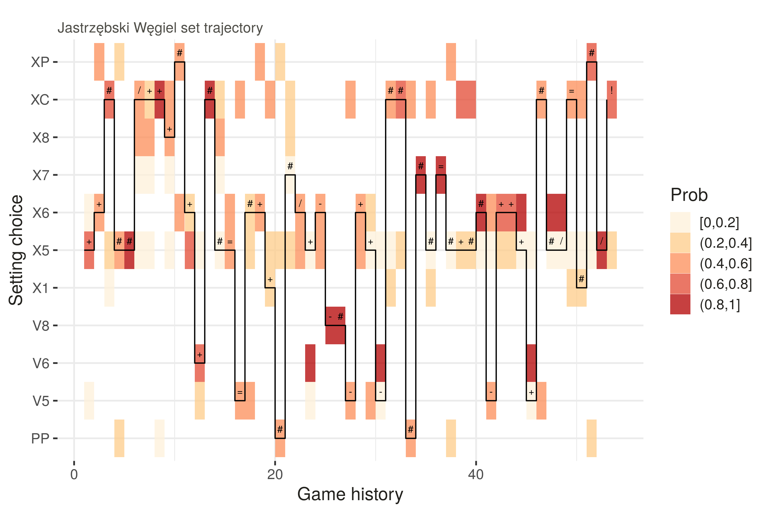
The plot shows the choices made by the bandit setter at each point over all of its simulations, and the probability of success that each one gave. The black line shows the choice that our real setter actually made for each point, along with its outcome (e.g. # was a kill, / was a blocked attack).
What can we say from this? Well, it does not seem that the setter departed too much from what our bandit setter would do, with a few exceptions. For example, in rally 37 the bandit found that a PP (setter dump) or XP (pipe) attack would have had the best chance of success, but our real setter chose an X5 (fast ball to position 4 — which in fact resulted in an attack kill).
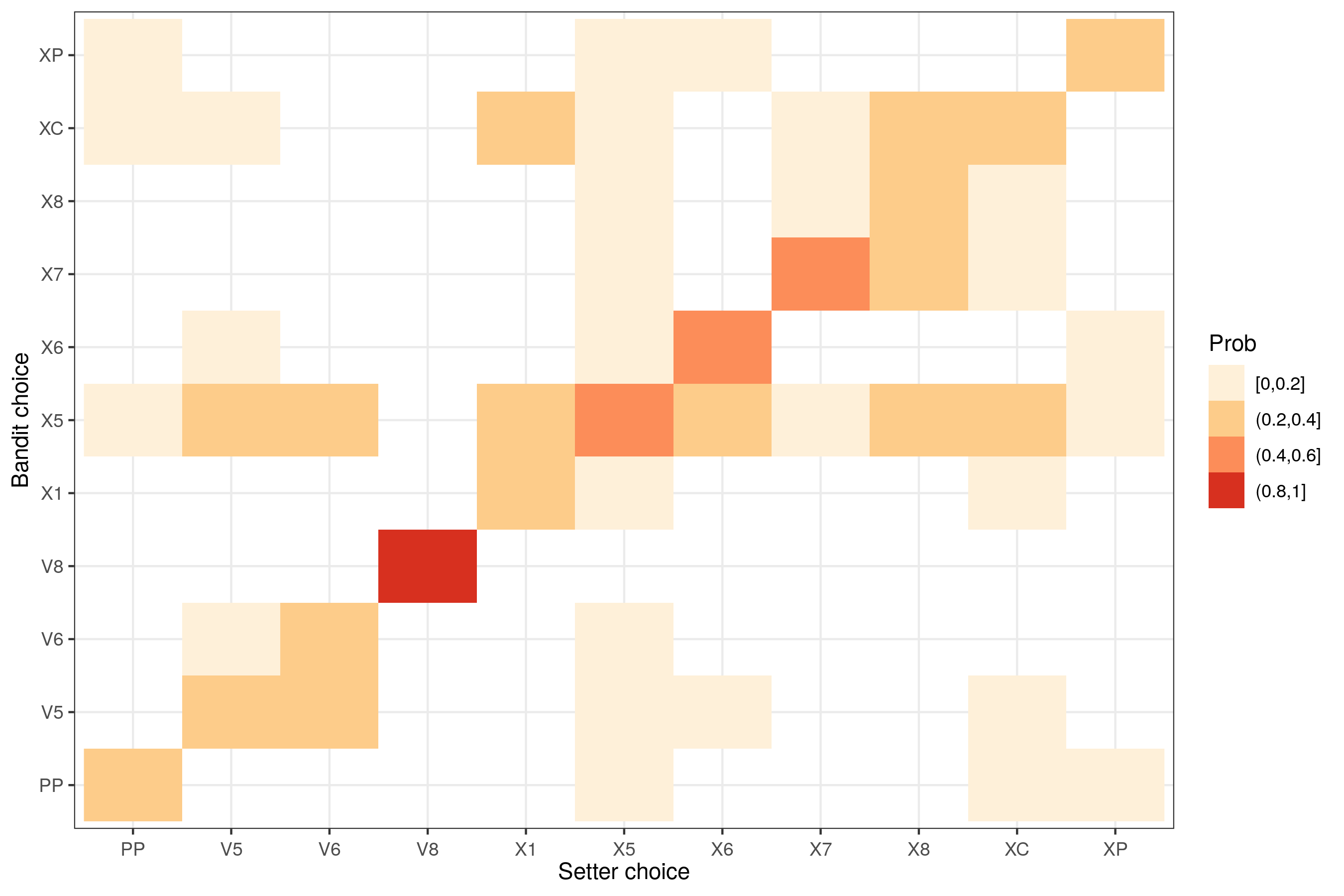
Finally, this last plot is a comparison between what the setter played, and what the bandit played. If they played identically, you’d only see dark colored squares on the diagonal. Which it is, mostly, with perhaps the exception of X1, where the bandit would also play XC and X5, and X8, where the bandit would play quicks and X5 … I will leave the interpretation to the people most familiar with that particular team, and that game…
Can we keep digging? Absolutely. But this has been a long post already, so we’ll do that in the next one!
Coming back to my very inquisitive player, maybe I need to actually give feedback about the setting options in front of the team, so they know for a fact that yes, I try to look at every aspect, and no, the setter does not have a blank check!!!
Additional considerations
As in any statistical model, some hypotheses/assumptions are made to project the complex world into a much more simplified version which we can quantify. In this instance, the following assumptions were made:
The kill rate (for a given reception quality, rotation, and attack code) is constant throughout the whole game. Using reception quality, rotation, AND attack code as the basis for this does have the effect of slicing the dataset into very small pieces and potentially making the results susceptible to outliers in the data. There might be better options, and this decision would also probably be test-able, in the statistical sense. Shall we explore that in another post?
Attacks have independent outcomes. In other words, the outcome of a given attack does not affect the outcome of the following attack
Now, the Bandit setter also assumes that a kill from an X5 attack (fast outside ball) when the setter is in position 3, from a perfect reception does not give any information on any other different attack outcome (where different means different call, different setter position or different pass quality). In a another post we will investigate if that can be changed, and some form of correlation introduced in the algorithm, in order to optimize its choice selection. (I’m assuming it will, and potentially we may be able to mimic a setter’s thought process… Maybe…)
The analysis code can be found in our ovlytics R package (look for the ov_simulate_setter_distribution and related functions).
You can also apply this analysis to your own data (without using R) via this app, which is part of the Science Untangled suite of volleyball analytics apps.