Our third and final submission to GBIF's Ebbe Nielsen Challenge in 2015.
Introduction
Unstructured data such as free text, images, sounds, and other media are less commonly used in biodiversity studies than structured information such as species occurrences. Nevertheless, these sources represent a rich stream of information, some of which is not generally available through more conventional sources. This information is of value for scientific, research, and conservation management use, as well as for communication and outreach to public and other audiences.
Species characteristics, or traits, are of interest to ecologists, in part because they provide a basis for mechanistic explanations of ecological phenomena1. Trait databases have been assembled (e.g. TraitBank, TRY, PanTHERIA) but detailed, quantitative species colour information is not commonly available, and studies of colour variation are relatively uncommon.
Species images are becoming increasingly available, due to a range of related factors including the rise of social media and photo sharing sites, increased support for digitization of collections from musea and other institutions, and the increased impetus to organise such media and make them freely available through networks such as GBIF. This submission converts a collection of images into quantitative data on species colouration, and then examines the taxonomic and spatial patterns in those data.
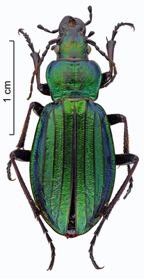
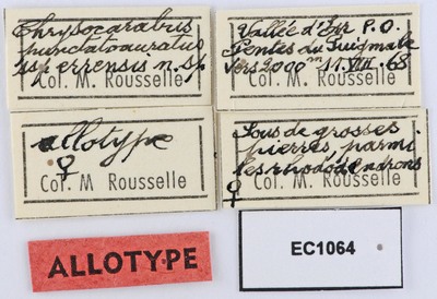
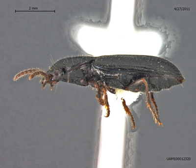
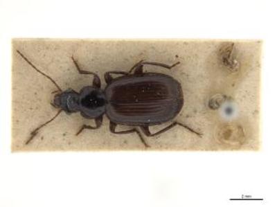
Images from collections are used here: these are typically more consistent (in terms of composition, lighting, and other details) than field photographs. Even so, analyses need to be able to cope with a range of issues and sources of variability. Some example specimen images are shown below, giving an indication of some of this variability:
 |
 |
| (a) | (b) |
 |
 |
| (c) | (d) |
Example of (a) a wonderful image, (b) label, (c) lateral view with difficult background, (d) difficult background
Source code
The code is available in two parts:
- The first part finds the list of species and their images, retrieves and caches the images, and extracts their colour palettes.
-
The example analyses shown in "Results" below. Extract these files into a suitable location and step your way through the beetle_colour_analyses.R code. Note for users not familiar with R: if you get errors saying "there is no package called blah" then you just need install the package:
install.packages("blah")
The first part (caching the images and extracting the palettes) is fairly slow, so the second link contains the data file from the first step. You can just start from here if you prefer.
Data processing
See the source code for details. Briefly, for the first step:
- Find the names of all of the species of interest: here, the family Carabidae (ground beetles).
- Find images for as many of these species as possible (up to 10 images per species), restricting ourselves to specimen images by specifying PRESERVED_SPECIMEN as the
basisOfRecordattribute. - Iterate through these images and build a global colour palette (i.e. a matrix of all of the colours present in all images). Colours are quantized (i.e. red/blue/green values, which can range from 0–1, are rounded to the nearest 0.05) in order to reduce the total number of colours, as well as helping to accommodate small variations in colour due to lighting and camera differences.
- Images are restricted to those that have near-white backgrounds. Unsuitable colours are also discarded: these are any that are white-ish or light-brownish (which are image backgrounds) or colours very close to black (which tend to be annotations or sometimes backgrounds). Discarding near-black colours does risk losing some pixels that are parts of specimens, but since black is the predominant beetle colour, it is unlikely to be of particular interest anyway.
Subsequent analyses are open-ended and could be driven by a range of scientific questions. Here, patterns with respect to taxonomy are examined, as well as spatial patterns. The spatial analyses are achieved by extracting occurrence data for the species of interest — the list of species present at a given location gives the corresponding colour palettes associated with that location.
As well as direct patterns in the colours, it is also possible to examine patterns in properties of the colour palettes. Various "property analyses" might be of interest — for example, patterns in individual colour channels (red, green, blue, or other channels such as hue when transformed to other colourspaces), or the relative probability of finding certain colours in the palette (e.g. where do beetles with red characteristics occur?)
Within-palette variability (i.e. how much variability is there within the colour palette of an individual species) is examined here as an example of a property analysis. Species with uniform colouration (e.g. all-black, or all-green) have low within-palette variability, whereas species with contrasting colours (e.g. black with green) have high values. Within-palette variability is calculated here using a dissimilarity approach: two colours are chosen at random from a given colour palette and their dissimilarity calculated, and this is repeated many times to find the average dissimilarity value for that palette.
Results
Through the GBIF API, 1029 images covering 190 of the 8736 Carabidae species were found. To supplement the results here, images were also sourced from the South Australian Museum collection (using almost the same source code, but using the ALA4R R package rather than rgbif). This yielded 1203 images covering 344 species. After reducing the images to those with near-white backgrounds (see methods above), the list was reduced to 346 images covering 158 species.
A sample of overall colour map (colours sampled with frequency proportional to their prevalence in the images) is shown below. There is clearly a predominance of brown and near-black colours, as expected, but also a range of greens, reds, yellows, and blues.
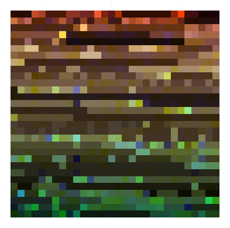 |
| A representative selection of colours from ground beetle specimen images |
With the basic results in hand (i.e. a colour palette for each species), there are a wealth of subsequent investigations that could be of interest. Some very preliminary analyses of patterns with respect to taxonomy and geography are presented here.
Colour patterns with taxonomy
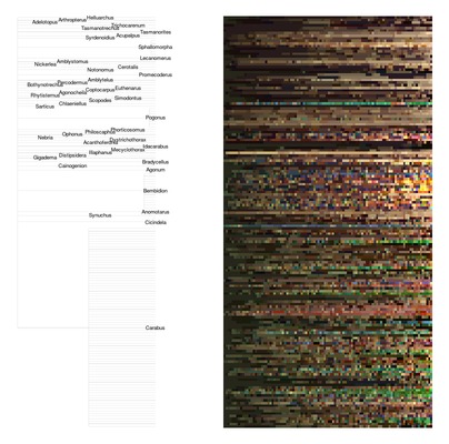
The figure below shows a taxonomic tree (genus and species within family; labels give genus), with samples from the corresponding colour palettes on the right. Some broad patterns are apparent: most of the greenish-bluish species lie within the Carabus genus, whereas those with yellow-orange tones are typically from Bembidion. Note that some of the yellowish-white colours may come from the heads of the specimen pins, which are present in most photographs (although these comprise a relatively small fraction of the image area).
Colour patterns in geographic space
A relatively simple method for depicting colour patterns in geographic space is to start by gridding up the region of interest. For each grid cell, occurrence data are used to find the species that are present, and then the colours in those species' colour palettes are sampled (with representative sampling weights, so that the more common colours are more prevalent in the sample).
Most of the occurrence data are from Europe and North America. For Europe, there appears to be a latitudinal gradient in colours, with green more prevalent in the south (e.g. France, Germany) and brown/dark orange through Scandinavia. Other, smaller scale patterns are also present, such as the region of blue, yellow, and brighter orange in the far north.
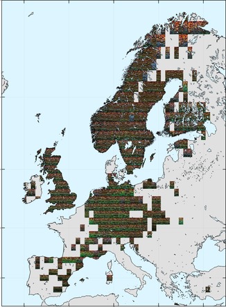 |
| Ground beetle colouration across Europe. Each tile in the image shows a representative sample of the colours of species present in that grid cell. Click for a higher-resolution version and zoom in. |
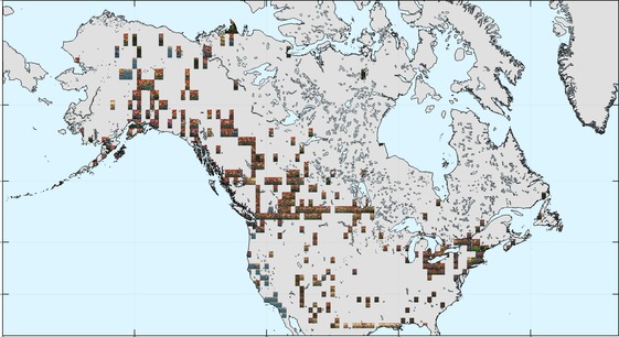
The occurrence data are sparser in North America, but similarly seem to have a more pronounced tendency towards orange hues at higher latitudes (through Canada and Alaska).
Maps derived directly from occurrence data are limited to the spatial coverage of that data (see "Further work", below). Spatial regression models can help to fill in gaps, by modelling a response variable as a function of environmental covariates. The example map below shows this idea: taxa with red colouration were identified, and then the probability of finding those taxa was modelled as a function of altitude, temperature, and rainfall conditions using a random forest model (see source code for details).
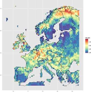 |
| Modelled probability of finding ground beetle taxa with red colouration, across Europe. Click for a higher-resolution version and zoom in. |
This map does bear some resemblance to the direct colour results, which is encouraging. Note, though, that the actual results in this example are probably not overly insightful. This is — at least in part — because the predictor variables were just conveniently-available bioclimatic variables, and not selected on the basis of any particularly good ecological reasoning. The partial dependence plots from the regression model could in principle be examined to deduce the environmental conditions associated with red beetles — these are not presented here for this reason (but see the source code for how to do this).
Colour palette properties
The within-species colour variability results (below) suggest that beetles in North America might generally have more variable colouration than in Europe. Areas of particularly low and particularly high colour-diversity may reflect sampling effort and data availability: see discussion below.
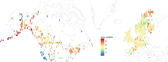 |
| Mean colour variability within ground beetle species across geographic space. Click for a higher-resolution version and zoom in. |
Further work
This work is merely a starting point: there is enormous scope for improvement in both the methods used and the specific results presented here.
Note that these preliminary analyses have been made without adult supervision — that is, no beetle ecologists or biologists were involved. Expert engagement would be an essential part of any further interpretation or refinement of these specific results, and so instead this discussion focuses on potential improvements to the methods.
Use of advanced image processing algorithms
The images used here were specifically chosen to be specimen images with consistent white or near-white backgrounds, so as to make the demonstration code more tractable. Undesirable images (e.g. of labels) were excluded automatically where possible (based on the file name of the image and the image colour palette characteristics) but manual exclusion of some such images was still required.
Relaxing the constraint on specimen-only images would lead to a much larger library of target images, broader taxonomic coverage, and potentially more robust results, but would in turn require more advanced processing techniques. The extra difficulties predominantly stem from the more-variable nature of the composition of such images — for example, the species in question is unlikely to be the only subject in the image, and will not be photographed from a consistent aspect (pose). Other sources of variability include lighting, weather conditions (rain, fog, bright sunshine), and camera equipment. However, if these difficulties can be overcome, the result will likely be a more general and more flexible set of tools, with a higher degree of automation, and ultimately greater benefit to the scientific community.
A relatively-recent but highly successful family of image processing algorithms are based on deep learning techniques such as convolutional neural networks. Software for these approaches — while still requiring considerable domain expertise to use effectively — is available (see e.g. Caffe and R-CNN). One of the difficulties is effectively training the networks. Worth noting is that pre-trained models are available online, and the Caffe web demonstration includes a "ground beetle" class — see this example screenshot:
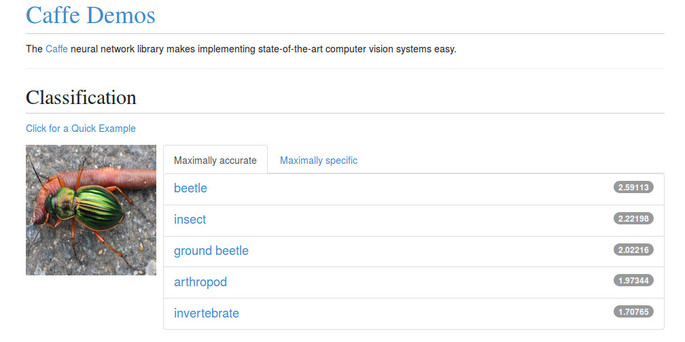 |
Thus — for the ground beetle application at least, and possibly others — there might be existing, trained models that can be used directly.
Object detection and image segmentation are also important, so that objects of interest can be automatically identified and delineated in photographs. See below for an example of bird detection from Zhang et al.2 (which actually goes further, detecting parts of objects, such as the head in this example).
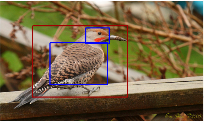 |
Other software libraries such as OpenCV are also candidates for improved image processing.
Downstream modelling
The maps shown above generally use the species occurrence records to directly infer the presence or absence of a species at a given location. Some of the patterns in the results are therefore likely to be reflections of patterns in sampling effort and data availability (e.g. spatial and taxonomic biases in occurrence records and images) rather than genuine biological patterns. An obvious solution to this issue to to use spatial modelling to better account for distribution of effort. One possible approach would be to construct a distribution model for each of the species of interest (i.e. estimate probability of presence as a function of environmental and other covariates). Given a location of interest, the species composition would then be estimated from the models, rather than inferred directly from occurrence data.
Alternatively, rather than modelling the species distributions (which would be a lot of work for many species), the modelling could be applied directly to properties of the colour palettes — e.g. modelling red/green/blue colour channel intensities as a function of environment, or modelling the colour composition directly (e.g. treating it as a multinomial distribution, as can be done for community-level modelling of species abundances3). The "probability of finding beetles with red colouration" is an example of this idea.
The within-palette variability example shows the use of a dissimilarity-style analysis. There is an enormous body of ecological research based on the concept of dissimilarities, and so many of these techniques (clustering, ordination, etc) could potentially be applied here. Some subtleties would need to be investigated: for example, the within-palette variability used a dissimilarity measure based on human perception of colour difference4. Models using colour perception of different animal groups might yield very different results.
Finally, colouration in beetles reflects various ecological phenomena, including camouflage, mimicry, or warnings to predators. Analyses that draw on other biological data (predator occurrences, for example) might be worth pursuing.
Footnotes:
e.g. Verbek W et al. (2013) Delivering on a promise: integrating species traits to transform descriptive community ecology into a predictive science. http://dx.doi.org/10.1899/12-092.1
Zhang N, Donahue J, Girshick R, Darrell T (2014) Part-based R-CNNs for Fine-grained Category Detection. European Conference on Computer Vision (ECCV), 2014. http://www.cs.berkeley.edu/~rbg/papers/part-rcnn.pdf
Arbel J, King C, Raymond B, Winsley T, Mengersen KL (submitted) Application of a Bayesian nonparametric model to derive toxicity estimates based on the response of Antarctic microbial communities to fuel contaminated soil. Ecology & Evolution

