
Timeouts: 2015/16 Italian League
Ben Raymond (ben@untan.gl), Mark Lebedew (@homeonthecourt)
This page gives the detailed breakdown of the analyses discussed in this post on Mark’s blog.
1 Data and software
All analyses have been conducted in R. An R package for reading and analyzing DataVolley scouting files is in development: see https://github.com/raymondben/datavolley.
The data are almost the entire set of matches (missing just one match) from the 2015/16 Italian League. A brief summary is given below.
Number of matches: 131
Match dates: 2015-01-11 to 2016-11-02
Number of individual players: 165
Number of data rows: 179156
Number of individual points: 22576
Number of serves: 22538
Number of timeouts: 1480
Number of technical timeouts: 471| Team | Played | Won | Win rate | Sets played | Sets won | Set win rate | Points for | Points against | Points ratio |
|---|---|---|---|---|---|---|---|---|---|
| Calzedonia Verona | 22 | 14 | 0.636 | 86 | 52 | 0.605 | 1956 | 1911 | 1.024 |
| CMC Romagna | 22 | 7 | 0.318 | 92 | 36 | 0.391 | 2001 | 2116 | 0.946 |
| Cucine Lube Civitanova | 21 | 19 | 0.905 | 79 | 61 | 0.772 | 1876 | 1618 | 1.159 |
| DHL Modena | 22 | 18 | 0.818 | 86 | 60 | 0.698 | 2003 | 1822 | 1.099 |
| Diatec Trentino | 22 | 17 | 0.773 | 85 | 55 | 0.647 | 1968 | 1770 | 1.112 |
| Exprivia Molfetta | 21 | 10 | 0.476 | 81 | 40 | 0.494 | 1786 | 1796 | 0.994 |
| Gi Group Monza | 22 | 7 | 0.318 | 85 | 33 | 0.388 | 1907 | 2022 | 0.943 |
| Ninfa Latina | 22 | 9 | 0.409 | 87 | 38 | 0.437 | 1897 | 1943 | 0.976 |
| Piacenza | 22 | 2 | 0.091 | 82 | 20 | 0.244 | 1678 | 1919 | 0.874 |
| Revivre Milano | 22 | 5 | 0.227 | 82 | 24 | 0.293 | 1723 | 1937 | 0.890 |
| Sir Safety Conad Perugia | 22 | 14 | 0.636 | 83 | 50 | 0.602 | 1912 | 1791 | 1.068 |
| Tonazzo Padova | 22 | 9 | 0.409 | 84 | 37 | 0.440 | 1869 | 1931 | 0.968 |
2 Timeouts
The motivation for this analysis is to examine the effects of timeouts in volleyball matches, particularly with respect to serve errors and sideouts.
2.1 General timeout patterns
We start with a general overview of timeout calling patterns. How often do different teams call timeouts?
Broadly speaking, teams that have a higher win rate (percentage of matches won) call less timeouts. A plot of this relationship is shown below:
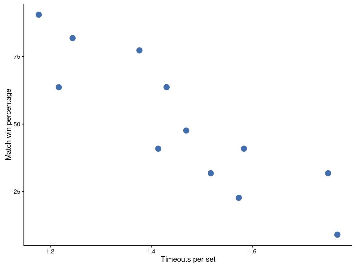
Figure 1: Timeouts per set plotted against match win percentage. Each point represents one team
Timeouts are almost universally called by the team that is not currently serving:
14 timeouts (of 1480 total) called by serving teamWhen are timeouts called? Below is a histogram of the opposing team’s score (at the time that each timeout was called). Sets 1–4 are plotted separately from set 5, for obvious reasons.
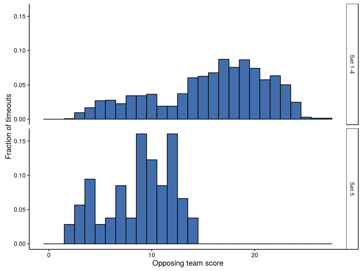
Figure 2: Histograms of timeouts against opposing team’s score
For sets 1–4, there are technical timeouts at 12 points, which correspond to the dip in the upper panel. Coaches will typically avoid using a team timeout when a technical timeout is imminent. This dip aside, there is a general increase in the number of timeouts called as the set progresses, peaking just below 20 points. Set 5 (during which there are no technical timeouts) shows a peak around 3–4 points, a second around 10 points, and possibly a third around 13 points.
This can be plotted with both the calling team’s score and the opposing team’s score. The colours in the plot below show the number of timeouts called for each combination of calling team’s score and opposing team’s score:
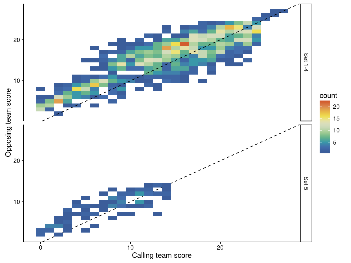
Figure 3: Heatmaps of timeouts against calling and opposing team scores
There is a hotspot when the opposing team’s score is around 5 and the calling team’s score is lower — so the opposition has jumped out to a quick start. It is clear that most timeouts generally lie above the 1:1 dashed line, meaning that the opposing team is ahead of the calling team. There are also a number of timeouts called when the calling team is ahead of the opposition, mostly towards the end of the set: possibly these might correspond to situations where the opposing team has scored a run of points and is catching up to the calling team, but this wasn’t looked at further here.
A simplified version of the previous graph is below, showing only the score differential (calling team’s score minus the opposing team’s score) when each timeout was called:
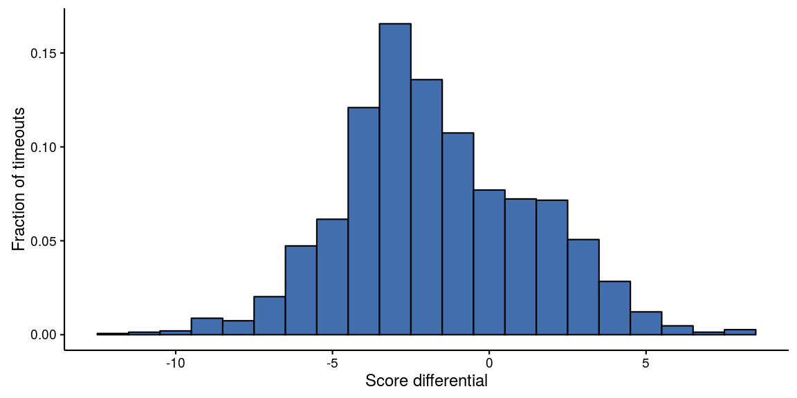
Figure 4: Histogram of timeout frequency as a function of score differential
Only a small proportion (about 24%) of timeouts were called by a team that was leading at the time.
None of the above is particularly surprising, but it serves to confirm that timeouts are generally called by the receiving team, at times when some sort of intervention might be expected to be helpful to the outcome.
2.2 Effect of timeouts on sideouts and serve effort
The following indicators of serve success and effort are considered:
- whether the serve was a jump serve or not. The data in fact provides “serve type”, which is one of jump, jump-float, float, or unknown serve type. However, the latter two categories make up a vanishingly small fraction of overall serves, and so “serve type” can be adequately treated by converting it to a binary indicator of whether the serve was a jump serve or not
- serve error rate (the proportion of serves where a service error was made)
- ace rate (the proportion of serves that were aces)
- perfect pass rate (the proportion of receptions rated as a “perfect pass”).
The following indicators of the performance of the receiving team are calculated:
- sideout rate. Sideouts are expressed from the perspective of the receiving team (i.e. a sideout is a reception where the receiving team wins the point)
- earned sideout rate (sideout rate excluding service errors)
- first ball sideout rate (proportion of receptions where the first attack by the receiving team was successful)
Indicators analogous to the sideout indicators, but expressed from the perspective of the serving team, are also calculated. These are referred to as:
- serve loss rate (the proportion of serves where the serving team lost the point)
- earned serve loss rate (serve loss rate excluding service errors)
- first ball serve loss rate (proportion of serves where the first attack by the receiving team was successful).
These indicators will be evaluated for each of the following situations:
- the first serve of a set
- the first serve following a technical timeout
- the first serve following a normal timeout
- all other serves.
Statistical tests have been conducted to evaluate whether a given indicator varies across the different situations. What does a significant result mean in this context? We are assuming that our dataset is a sample that is representative of some larger volleyball universe. The significance (p-value) of a test performed on our data indicates the degree to which we expect the result in question to hold true in the larger universe.
The statistical models used here are generally binomial mixed-effects models, in which the response is the indicator in question, and a random effect by individual player is included. A “binomial” model simply means that the response can take one of two values (e.g. if we are examining serve errors, then a given serve was either an error or it was not). The random effect allows individual players to vary in their performance. Including this random term will also account for the fact that some players might perform the skill in question more often than others across the various serve categories.
In general, we test by fitting two models for each indicator. The first model has a single fixed predictor term (the serve category). The second has no predictor terms — that is, it assumes that the indicator does not vary with serve category. We then compare the fits of the two models. If the first model is a statistically better fit to the data (p<0.05), then it supports the idea that the indicator does indeed vary with serve category.
2.2.1 Results
Below is a tabulation of the number of individual players associated with each of the serve categories, and the average number of serves that each player made in that category.
| Serve category | Number of unique servers | Average number of serves per server |
|---|---|---|
| General play | 145 | 138.545 |
| First of set | 73 | 6.932 |
| Followed timeout | 126 | 11.730 |
| Followed technical timeout | 105 | 4.486 |
Notice that the “first serve of the set” category represents a much more limited number of players than the other categories. This is of course because the starting rotation of each team is relatively consistent from set to set. The number of players associated with serves after technical timeouts is next smallest, because technical timeouts occur at fixed scores (first team to 8 and 16 points) thus restricting the possible rotations that can occur at these times.
For each indicator a brief summary of the data is shown, along with “raw” and model estimates of rates. The raw rate is calculated directly from the data (e.g. number of errors divided by number of serves), whereas the model estimate is the same rate but adjusted by the random effect in the model for the individual players involved.
2.2.1.1 Serve error rate
The proportion of serves where a service error was made.
| Serve category | Serves | Errors | Raw serve error rate from data | Serve error rate model estimate |
|---|---|---|---|---|
| General play | 20089 | 3331 | 0.166 | 0.160 |
| First of set | 506 | 51 | 0.101 | 0.101 |
| Followed timeout | 1478 | 253 | 0.171 | 0.162 |
| Followed technical timeout | 471 | 66 | 0.140 | 0.136 |
Is there an overall difference in the service error rate in the various serve categories?
Significance of the serve category term: p=0.001
2.2.1.2 Ace rate
The proportion of serves that were aces.
| Serve category | Serves | Aces | Raw ace rate from data | Ace rate model estimate |
|---|---|---|---|---|
| General play | 20089 | 1184 | 0.059 | 0.054 |
| First of set | 506 | 18 | 0.036 | 0.034 |
| Followed timeout | 1478 | 85 | 0.058 | 0.050 |
| Followed technical timeout | 471 | 26 | 0.055 | 0.050 |
Significance of the serve category term: p=0.194
2.2.1.3 Perfect pass rate
The proportion of receptions that were rated as a perfect pass.
| Serve category | Receptions | Perfect passes | Raw perfect pass rate from data | Perfect pass rate model estimate |
|---|---|---|---|---|
| General play | 16758 | 3908 | 0.233 | 0.224 |
| First of set | 455 | 129 | 0.284 | 0.266 |
| Followed timeout | 1225 | 283 | 0.231 | 0.229 |
| Followed technical timeout | 405 | 85 | 0.210 | 0.205 |
Significance of the serve category term: p=0.150
The model in this case has an additional random term for the serving player (that is, it tries to account for idiosyncrasies in both the serving player’s serving ability as well as the receiving player’s passing ability).
2.2.1.4 Sideout rate
For sideout indicators, the result is modelled in the same way as before (binomial mixed model) but with a random effect on team rather than individual player (because the sideout rate most likely depends more heavily on the overall team, rather than just the player who is serving).
| Serve category | Serves | Sideouts | Raw sideout rate from data | Sideout rate model estimate |
|---|---|---|---|---|
| General play | 20089 | 13428 | 0.668 | 0.670 |
| First of set | 506 | 322 | 0.636 | 0.636 |
| Followed timeout | 1478 | 1008 | 0.682 | 0.685 |
| Followed technical timeout | 471 | 294 | 0.624 | 0.630 |
Significance of the serve category term: p=0.055
2.2.1.5 Earned sideout rate
Sideout and serve loss rates excluding service errors (i.e. where the receiving team “earned” the sideout).
| Serve category | Receptions | Earned sideouts | Raw earned sideout rate from data | Earned sideout rate model estimate |
|---|---|---|---|---|
| General play | 16758 | 10097 | 0.603 | 0.604 |
| First of set | 455 | 271 | 0.596 | 0.595 |
| Followed timeout | 1225 | 755 | 0.616 | 0.620 |
| Followed technical timeout | 405 | 228 | 0.563 | 0.568 |
Significance of the serve category term: p=0.309
2.2.1.6 First ball sideout rate
Proportion of receptions where the first attack by the receiving team was successful (service errors are excluded).
| Serve category | Receptions | First ball sideouts | Raw first ball sideout rate from data | First ball sideout rate model estimate |
|---|---|---|---|---|
| General play | 16758 | 7234 | 0.432 | 0.432 |
| First of set | 455 | 200 | 0.440 | 0.438 |
| Followed timeout | 1225 | 543 | 0.443 | 0.446 |
| Followed technical timeout | 405 | 161 | 0.398 | 0.400 |
Significance of the serve category term: p=0.457
2.2.1.7 Jump serve rate
In this case a simpler model is used, with no random effect by player, because players tend to be consistent in whether they jump serve or not (which causes problems in the numerical fitting of the model).
| Serve category | Serves | Jump serves | Raw jump serve rate from data | Jump serve rate model estimate |
|---|---|---|---|---|
| General play | 20089 | 12405 | 0.618 | 0.618 |
| First of set | 506 | 291 | 0.575 | 0.575 |
| Followed timeout | 1478 | 937 | 0.634 | 0.634 |
| Followed technical timeout | 471 | 277 | 0.588 | 0.588 |
Significance of the serve category term: p=0.066
2.3 Timeouts over the course of a set
In the previous section we found little evidence to support the idea that overall sideout rate differs after timeout than during general play. Are there more subtle effects — for example, does the effectiveness of a timeout change as a set progresses? Here we are focusing on sideout rate, and only comparing after-timeout serves to all other serves.
2.3.1 Set score
Does sideout rate vary over the course of a set? The data are summarised below. The lines show the mean sideout rates and the shaded bands their 95% confidence intervals, for different values of “score” (where “score” here means the higher of the two teams’ scores at the beginning of the rally):
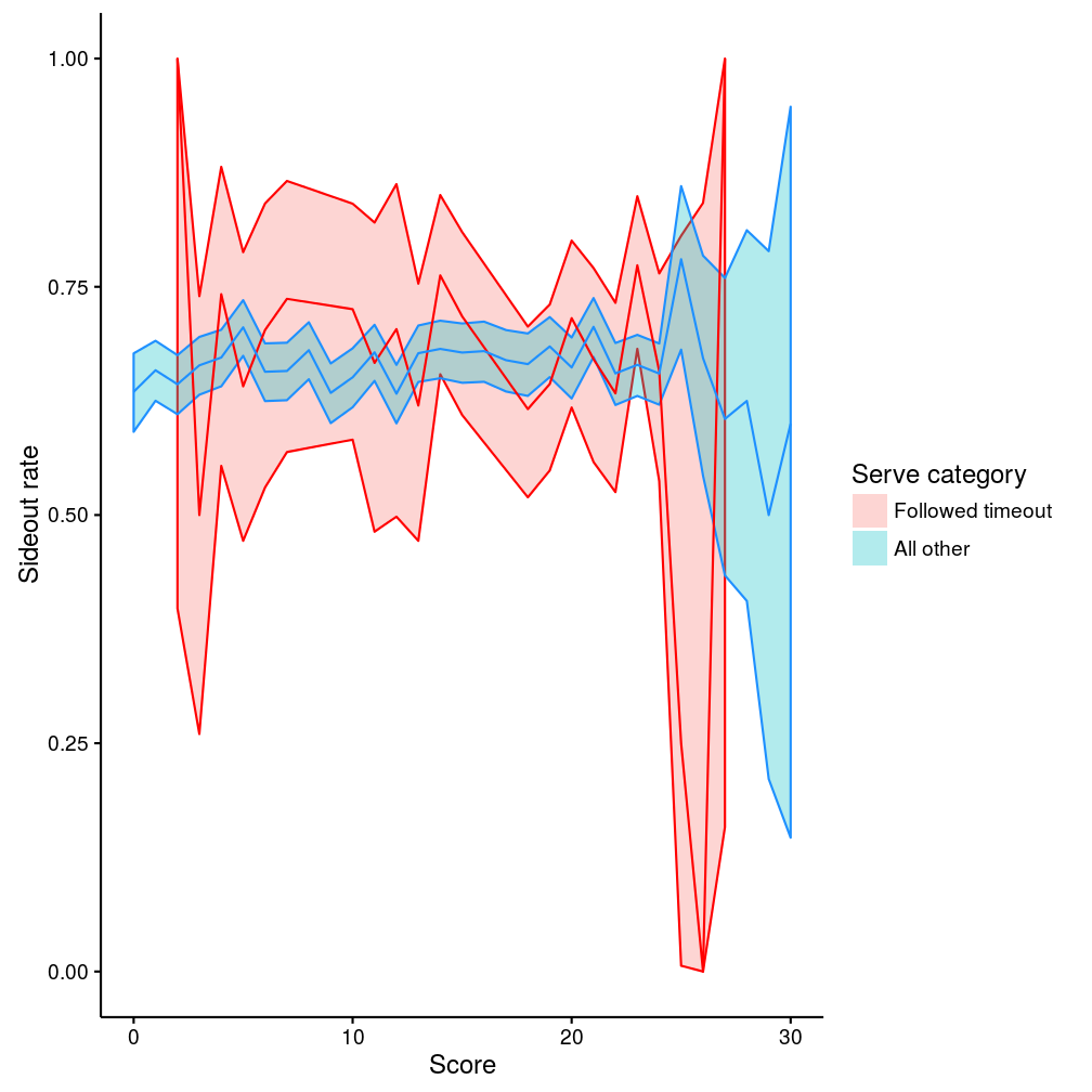
Figure 5: Sideout rate by set score
During non-timeout play (blue line) the sideout rate is clearly pretty constant. The after-timeout rate (red line) is very similar to the blue line. The shaded bands are wider, indicating that we are less confident in our estimate (because there are less data for after-timeout serves than for other serves), but there is no substantive difference between the two lines. (The big dip in the red line around 25 points is an artifact from a lack of data in this region.)
2.3.2 Score differential
What about score differential? Here, differential is defined relative to the serving team (so a positive score differential means that the serving team is ahead). We don’t distinguish which team called a timeout (though as previously shown it’s overwhelmingly the receiving team).
The data are summarised below (the lines show the mean sideout rates and the shaded bands their 95% confidence intervals):
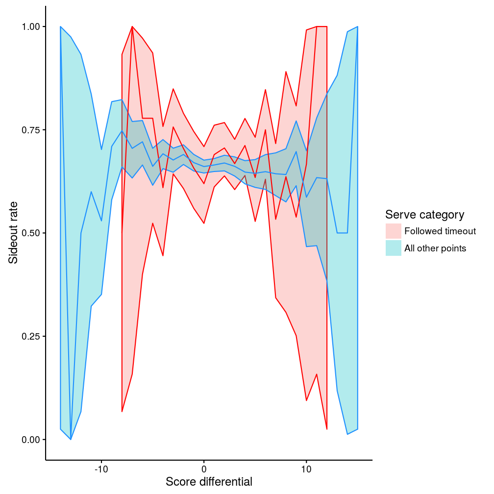
Figure 6: Sideout rate by score differential
For score differential between about -10 and +10, the two lines are again very similar. Overall, the confidence intervals of the two curves overlap, consistent with out earlier finding that there is no overall difference in sideout rate after timeout. Sideout rate is higher when the serving team is behind, and sideout rate is lower when the serving team is ahead (exactly as one would expect). At more extreme score differentials (below -10 or above +10) the data are less consistent and the confidence intervals much wider, indicating that there isn’t sufficient data to draw strong conclusions.
If we are prepared to assume that sideout rate should vary smoothly as a function of score differential, then we can fit a model, and this shows the relationships a little more clearly (a generalised additive model with smoothing spline was used here):
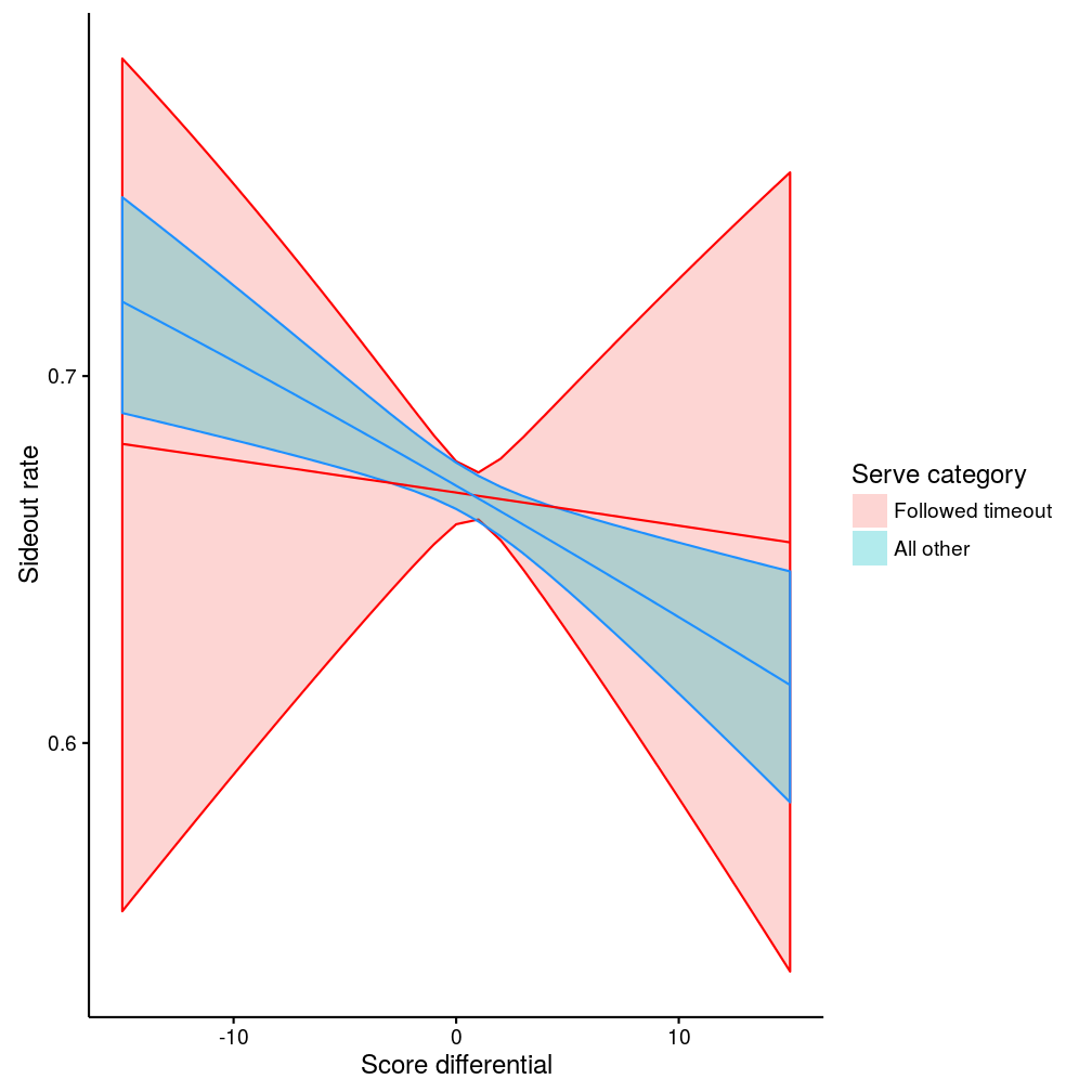
Figure 7: Sideout rate by score differential, from smoothed model
3 Serve runs
First find runs of serves, and tabulate how many runs we have of length 1, 2, 3, etc. The answer can be compared to the answer that we would expect given our overall sideout rate (we know that our overall sideout rate is 67% — so we expect 67% of serve runs to be of length 1. Runs of length two must occur when the first serve is not sided out but the second is, which will happen with frequency (1-0.67)*0.67, or about 22% of serve-runs. And so on):
| Serve run length | Fraction of serve runs | Fraction expected |
|---|---|---|
| 1 | 0.677 | 0.668 |
| 2 | 0.220 | 0.222 |
| 3 | 0.070 | 0.074 |
| 4 | 0.021 | 0.025 |
| 5 | 0.007 | 0.008 |
| 6 | 0.003 | 0.003 |
| 7 | 0.001 | 0.001 |
| 8 | 0.000 | 0.000 |
| 9 | 0.000 | 0.000 |
So the numbers we are extracting from the data are about right. The small differences are at least partly due to the ends of sets (say a set finishes with a run of three serves: we do not count this as a run of three because it didn’t end with a sideout — maybe it would have continued for several more serves had the end of the set not brought it to a premature halt).
Now we can look at serve error and sideout rates according to the positions of serves in their runs (e.g. is a serve error more likely on the first serve in a run compared to the second, for example). We only consider runs up to five serves in length, to keep the output manageable (and as can be seen from the above table, runs greater than five in length represent only a very small fraction of serve runs). Data summary:
| Team | Run position | Number of serves | Number of serve errors | Serve error rate |
|---|---|---|---|---|
| ALL TEAMS | 1 | 15290 | 2399 | 0.157 |
| ALL TEAMS | 2 | 4919 | 873 | 0.177 |
| ALL TEAMS | 3 | 1563 | 285 | 0.182 |
| ALL TEAMS | 4 | 495 | 95 | 0.192 |
| ALL TEAMS | 5 | 177 | 30 | 0.169 |
We fit a model of serve error as a function of run position, so that we can examine whether serve error varies depending on where the serve is in its run. The model estimates for serve error rate should roughly match the values in the “ALL TEAMS” data summaries above, but will not necessarily match exactly because the model includes a random effect for the individual server (to try and account for variations due to individual servers).
| Run position | Serve error rate model estimate |
|---|---|
| 1 | 0.151 |
| 2 | 0.173 |
| 3 | 0.181 |
| 4 | 0.192 |
| 5 | 0.170 |
Significance of the run position term: p<0.001
We can do the same thing for sideout rate as a function of run position:
| Team | Run position | Number of serves | Number of sideouts | Sideout rate |
|---|---|---|---|---|
| ALL TEAMS | 1 | 15290 | 10209 | 0.668 |
| ALL TEAMS | 2 | 4919 | 3300 | 0.671 |
| ALL TEAMS | 3 | 1563 | 1055 | 0.675 |
| ALL TEAMS | 4 | 495 | 314 | 0.634 |
| ALL TEAMS | 5 | 177 | 108 | 0.610 |
| Run position | Sideout rate model estimate |
|---|---|
| 1 | 0.668 |
| 2 | 0.673 |
| 3 | 0.679 |
| 4 | 0.640 |
| 5 | 0.618 |
Significance of the run position term: p=0.278
3.1 Timeouts
What about timeouts? Does calling a timeout during a run of serves affect the serve error or sideout rate? First of all, we fit the same models as above, but with an additional term for whether or not the serve followed a timeout. That is, the serve error/sideout rate is estimately separately for each run position, along with an additional adjustment for timeout. The timeout adjustment applies equally to all serve run positions.
| Factor level | Serve error rate model estimate (General play) | Serve error rate model estimate (Followed timeout) |
|---|---|---|
| Run position 1 | 0.152 | 0.140 |
| 2 | 0.175 | 0.162 |
| 3 | 0.185 | 0.171 |
| 4 | 0.203 | 0.188 |
| 5 | 0.170 | 0.157 |
Significance of the timeout term: p=0.217
Note that the error rate estimates here (for run position 1–5) are slightly different than in the previous model — because now we are additionally accounting for the effect of timeouts.
| Factor level | Sideout rate model estimate (General play) | Sideout rate model estimate (Followed timeout) |
|---|---|---|
| Run position 1 | 0.670 | 0.688 |
| 2 | 0.671 | 0.689 |
| 3 | 0.673 | 0.691 |
| 4 | 0.640 | 0.659 |
| 5 | 0.622 | 0.641 |
Significance of the timeout term: p=0.176
These two models assume that timeouts affect all serves equally. Perhaps we believe that timeouts might affect serve error rate differently depending on the serve run position (for example, we might think that a timeout after one successful serve will not have any effect, but a timeout after a run of two serves might). We can also test this, but this time we need to fit a model that estimates a separate error rate for each run position, both during normal play and after timeout. In this case, rather than try and show the data summary (it is becoming rather complex) we just show the comparison of the two models:
## Data: srunxt
## Models:
## mfit_sretm: error ~ run_position + serve_category + (1 | player_name)
## mfit_sreti: error ~ run_position * serve_category + (1 | player_name)
##            Df   AIC   BIC logLik deviance Chisq Chi Df Pr(>Chisq)
## mfit_sretm  7 18825 18881  -9405    18811
## mfit_sreti 11 18829 18916  -9403    18807  4.28      4       0.37
And for sideout rate:
## Data: srunxt
## Models:
## mfit_srsotm: serve_loss ~ run_position + serve_category + (1 | team)
## mfit_srsoti: serve_loss ~ run_position * serve_category + (1 | team)
##             Df   AIC   BIC logLik deviance Chisq Chi Df Pr(>Chisq)
## mfit_srsotm  7 27220 27276 -13603    27206
## mfit_srsoti 11 27225 27313 -13602    27203  3.35      4        0.5
We can double-check this by eyeballing the data, and by explicitly testing the effect of sideout at each position in the serve run (i.e. fitting a new model for each serve run position, and testing whether timeout has a significant effect). In this case we only compare post-timeout serves to serves during general play (i.e. not using data from serves after technical timeouts or first serve of a set). Compare the “Sideout rate (general play)” and “Sideout rate (followed timeout)” columns in the following table:
| Run position | Number of serves (general play) | Number of sideouts (general play) | Sideout rate (general play) | Number of serves (followed timeout) | Number of sideouts (followed timeout) | Sideout rate (followed timeout) | Significantly different from general play |
|---|---|---|---|---|---|---|---|
| 1 | 14310 | 9570 | 0.669 | 196 | 144 | 0.735 | 0.036 |
| 2 | 4084 | 2740 | 0.671 | 728 | 492 | 0.676 | 0.773 |
| 3 | 1132 | 757 | 0.669 | 382 | 264 | 0.691 | 0.418 |
| 4 | 349 | 225 | 0.645 | 124 | 78 | 0.629 | 0.755 |
| 5 | 131 | 81 | 0.618 | 37 | 23 | 0.622 | 0.983 |
3.2 Calling timeouts during serve runs
When during serve runs are timeouts called? After how many breakpoints (points won on serve)?
| Number of breakpoints | Number of serves | Number of timeouts | Timeout rate |
|---|---|---|---|
| 0 | 15290 | 196 | 0.013 |
| 1 | 4919 | 728 | 0.148 |
| 2 | 1563 | 382 | 0.244 |
| 3 | 495 | 124 | 0.251 |
| 4 | 177 | 37 | 0.209 |
Are multiple timeouts ever called during a single serve run?
Rarely. There were 1436 serve runs in which at least one timeout was called. Two timeouts were called in only 42 of these.